Revisiting k-Means: 3 Approaches to Make It Work Better

Revisiting k-Means: 3 Approaches to Make It Work Better
Image by Author | ChatGPT

Introduction

The k-means algorithm is a cornerstone of unsupervised machine learning, known for its simplicity and trusted for its efficiency in partitioning data into a predetermined number of clusters. Its straightforward approach — assigning data points to the nearest centroid and then updating the centroid based on the mean of the assigned points — makes it one of the first algorithms most data scientists learn. It is a workhorse, capable of providing quick and valuable insights into the underlying structure of a dataset.

This simplicity comes with a set of limitations, however. Standard k-means often struggles when faced with the complexities of real-world data. Its performance can be sensitive to the initial placement of centroids, it requires the number of clusters to be specified in advance, and it fundamentally assumes that clusters are spherical and evenly sized. These assumptions rarely hold true in the wild, leading to suboptimal or even misleading results.

Fortunately, over the many years that k-means has been relied upon, the data science community has developed several clever modifications and extensions to address these shortcomings. These one-time hacks, but now core extensions, enhance the robustness and applicability of k-means, transforming it from a simple textbook algorithm into a tool for practical data analysis.

This tutorial will explore three of the most effective techniques to make k-means work better in the wild, specifically:

Using k-means++ for smarter centroid initialization
Leveraging the silhouette score to find the optimal number of clusters
Applying the kernel trick to handle non-spherical data

Let’s get started.

1. Smarter Centroid Initialization with k-means++

One of the greatest weaknesses of the standard k-means algorithm is its reliance on random centroid initialization. A poor initial placement of centroids can lead to several problems, including converging to a suboptimal clustering solution and requiring more iterations to achieve convergence, which then increases computation time. Imagine a scenario where all initial centroids are randomly placed within a single, dense region of data — the algorithm might struggle to correctly identify distinct clusters located further away. This sensitivity means that running the same k-means algorithm on the same data can produce different results each time, making the process less reliable.

The k-means++ algorithm was introduced to overcome this. Instead of purely random placement, k-means++ uses a smarter, still probabilistic method to seed the initial centroids. The process starts by choosing the first centroid randomly from the data points. Then, for each subsequent centroid, it selects a data point with a probability proportional to its squared distance from the nearest existing centroid. This procedure inherently favors points that are further away from the already chosen centers, leading to a more dispersed and strategic initial placement. This approach increases the likelihood of finding a better final clustering solution and often reduces the number of iterations needed for convergence.

Implementing this in practice is remarkably simple, as most modern machine learning libraries — including Scikit-learn — have integrated k-means++ as the default initialization method. By simply specifying init="k-means++", you can leverage this approaches without any complex coding.

from sklearn.cluster import KMeans from sklearn.datasets import make_blobs # Generate sample data X, y = make_blobs(n_samples=10000, n_features=10, centers=5, cluster_std=2.0, random_state=42) # Standard k-means with k-means++ initialization kmeans_plus = KMeans(n_clusters=5, init=”k-means++”, n_init=1, random_state=42) kmeans_plus.fit(X) # For comparison, standard k-means with random initialization kmeans_random = KMeans(n_clusters=5, init=”random”, n_init=1, random_state=42) kmeans_random.fit(X) print(f”k-means++ inertia: {kmeans_plus.inertia_}”) print(f”Random initialization inertia: {kmeans_random.inertia_}”)

from sklearn.cluster import KMeans

from sklearn.datasets import make_blobs

# Generate sample data

X, y = make_blobs(n_samples=10000,

n_features=10,

centers=5,

cluster_std=2.0,

random_state=42)

# Standard k-means with k-means++ initialization

kmeans_plus = KMeans(n_clusters=5, init=‘k-means++’, n_init=1, random_state=42)

kmeans_plus.fit(X)

# For comparison, standard k-means with random initialization

kmeans_random = KMeans(n_clusters=5, init=‘random’, n_init=1, random_state=42)

kmeans_random.fit(X)

print(f“k-means++ inertia: {kmeans_plus.inertia_}”)

print(f“Random initialization inertia: {kmeans_random.inertia_}”)

Output:

k-means++ inertia: 400582.2443257831 Random initialization inertia: 664535.6265023422

k–means++ inertia: 400582.2443257831

Random initialization inertia: 664535.6265023422

As indicated by the differences in inertia — the sum of squared distances of data points to their centroid — k-means++ outperforms random initialization significantly in this case.

2. Finding the Optimal Number of Clusters with the Silhouette Score

An obvious limiting challenge with k-means is the requirement that you to specify the number of clusters, k, before running the algorithm. In many real-world scenarios, the optimal number of clusters is not known ahead of time. Choosing an incorrect k can lead to either over-segmenting the data into meaningless micro-clusters or under-segmenting it by grouping distinct patterns together. While methods to help determine the optimal number of clusters like the “elbow method” exist, they can be ambiguous and difficult to interpret, especially when there isn’t a clear “elbow” in the visual plot of variance.

A more robust and quantitative approach is to use the silhouette score. This metric provides a way to evaluate the quality of a given clustering solution by measuring how well-separated the clusters are. For each data point, the silhouette score is calculated based on two values:

cohesion – the average distance to other points in the same cluster
separation – and the average distance to points in the nearest neighboring cluster

Essentially, we are measuring how similar data points are to other data points in their own cluster, and how different they are from data points in other clusters, which, intuitively, are exactly what a successful k-means clustering solution should be maximizing.

Theese scores range from -1 to +1, where a high value indicates that the point is well-matched to its own cluster and poorly matched to neighboring clusters.

To find the optimal k, you can run the k-means algorithm for a range of different k values and calculate the average silhouette score for each. The value of k that yields the highest average score is typically considered the best choice. This method provides a more data-driven way to determine the number of clusters, moving beyond simple heuristics and enabling a more confident selection.

Let’s see the results of calculating the silhouette score for a range of k values from 2 to 10 using Scikit-learn, determine which value is the best, and plotting the results to compare to these results.

from sklearn.cluster import KMeans from sklearn.metrics import silhouette_score from sklearn.datasets import make_blobs import matplotlib.pyplot as plt # Generate sample data X, y = make_blobs(n_samples=10000, n_features=10, centers=5, cluster_std=2.0, random_state=42) # Determine optimal k (from 2 to 10) using silhouette score silhouette_scores = [] k_values = range(2, 11) for k in k_values: kmeans = KMeans(n_clusters=k, init=”k-means++”, n_init=10, random_state=42) kmeans.fit(X) score = silhouette_score(X, kmeans.labels_) silhouette_scores.append(score) print(f”For k = {k}, the silhouette score is {score:.4f}”) # Find the optimal k and best score best_score = max(silhouette_scores) optimal_k = k_values[silhouette_scores.index(best_score)] # Output final results print(f”\nThe optimal number of clusters (k) is: {optimal_k}”) print(f”This was determined by the highest silhouette score of: {best_score:.4f}”) # Visualizing the results plt.figure(figsize=(10, 6)) plt.plot(k_values, silhouette_scores, marker=”o”) plt.title(‘Silhouette Scores for Various Numbers of Clusters’) plt.xlabel(‘Number of clusters (k)’) plt.ylabel(‘Silhouette score’) plt.xticks(k_values) plt.grid(True) plt.show()

from sklearn.cluster import KMeans

from sklearn.metrics import silhouette_score

from sklearn.datasets import make_blobs

import matplotlib.pyplot as plt

# Generate sample data

X, y = make_blobs(n_samples=10000,

n_features=10,

centers=5,

cluster_std=2.0,

random_state=42)

# Determine optimal k (from 2 to 10) using silhouette score

silhouette_scores = []

k_values = range(2, 11)

for k in k_values:

kmeans = KMeans(n_clusters=k, init=‘k-means++’, n_init=10, random_state=42)

kmeans.fit(X)

score = silhouette_score(X, kmeans.labels_)

silhouette_scores.append(score)

print(f“For k = {k}, the silhouette score is {score:.4f}”)

# Find the optimal k and best score

best_score = max(silhouette_scores)

optimal_k = k_values[silhouette_scores.index(best_score)]

# Output final results

print(f“\nThe optimal number of clusters (k) is: {optimal_k}”)

print(f“This was determined by the highest silhouette score of: {best_score:.4f}”)

# Visualizing the results

plt.figure(figsize=(10, 6))

plt.plot(k_values, silhouette_scores, marker=‘o’)

plt.title(‘Silhouette Scores for Various Numbers of Clusters’)

plt.xlabel(‘Number of clusters (k)’)

plt.ylabel(‘Silhouette score’)

plt.xticks(k_values)

plt.grid(True)

plt.show()

Output:

For k = 2, the silhouette score is 0.4831 For k = 3, the silhouette score is 0.4658 For k = 4, the silhouette score is 0.5364 For k = 5, the silhouette score is 0.5508 For k = 6, the silhouette score is 0.4464 For k = 7, the silhouette score is 0.3545 For k = 8, the silhouette score is 0.2534 For k = 9, the silhouette score is 0.1606 For k = 10, the silhouette score is 0.0695 The optimal number of clusters (k) is: 5 This was determined by the highest silhouette score of: 0.5508

For k = 2, the silhouette score is 0.4831

For k = 3, the silhouette score is 0.4658

For k = 4, the silhouette score is 0.5364

For k = 5, the silhouette score is 0.5508

For k = 6, the silhouette score is 0.4464

For k = 7, the silhouette score is 0.3545

For k = 8, the silhouette score is 0.2534

For k = 9, the silhouette score is 0.1606

For k = 10, the silhouette score is 0.0695

The optimal number of clusters (k) is: 5

This was determined by the highest silhouette score of: 0.5508

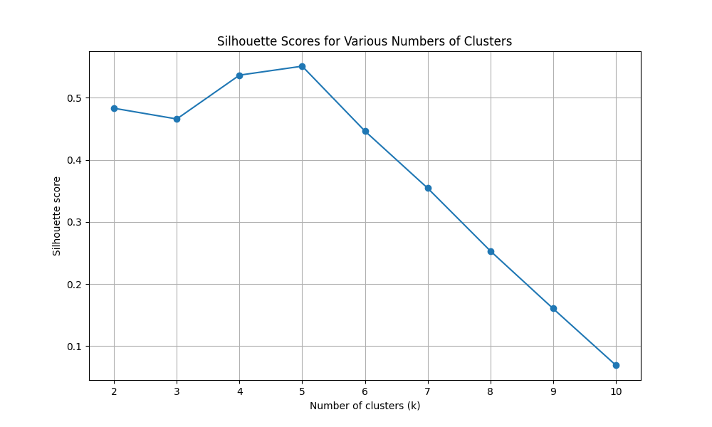
Figure 1: Silhouette scores for various numbers of clusters (for k values from 2 to 10)

We can see that 5 is the optimal k value with a silhouette score of 0.5508.

3. Handling Non-Spherical Clusters with Kernel k-Means

Perhaps the most frustrating and unrealistic limitations of k-means is its assumption that clusters are convex and isotropic, meaning they are roughly spherical and have similar sizes. This is because k-means defines clusters based on the distance to a central point, which inherently creates sphere-like boundaries. When faced with real-world data that contains complex, elongated, or non-linear shapes, standard k-means fails to identify these patterns correctly. For example, it would be unable to separate two concentric rings of data points, as it would likely split them with a straight line.

To address this, we can employ the kernel trick, a concept central to the workings of support vector machines. Kernel k-means works by implicitly projecting the data into a higher-dimensional space where the clusters may become linearly separable or more spherical. This is done using a kernel function, such as the radial basis function (RBF), which computes the similarity between data points in this higher-dimensional space without ever having to explicitly calculate their new coordinates. By operating in this transformed feature space, kernel k-means can identify clusters with complex, non-spherical shapes that would not be possible for the standard algorithm to detect.

While Scikit-learn doesn’t have a direct KernelKMeans implementation, its SpectralClustering algorithm provides a powerful alternative that effectively achieves a similar outcome. Spectral clustering uses the connectivity of the data to form clusters and is particularly effective at finding non-convex clusters. It can be seen as a form of kernel k-means and serves as an excellent tool for this purpose. Let’s take a look.

from sklearn.cluster import KMeans, SpectralClustering from sklearn.datasets import make_moons import matplotlib.pyplot as plt # Generate non-spherical data X, y = make_moons(n_samples=500, noise=0.05, random_state=42) # Visualize the non-spherical data plt.figure(figsize=(8, 6)) plt.scatter(X[:, 0], X[:, 1], color=”blue”, s=15) # Add titles and labels for clarity plt.title(‘Sample Non-Spherical Data’) plt.xlabel(‘Feature 1’) plt.ylabel(‘Feature 2′) plt.grid(True, linestyle=”–“, alpha=0.6) plt.show() # Apply standard k-means kmeans = KMeans(n_clusters=2, n_init=10, random_state=42) kmeans_labels = kmeans.fit_predict(X) # Apply spectral clustering (as an alternative for kernel k-means) spectral = SpectralClustering(n_clusters=2, affinity=’nearest_neighbors’, random_state=42) spectral_labels = spectral.fit_predict(X) # Visualizing the results fig, (ax1, ax2) = plt.subplots(1, 2, figsize=(14, 6)) ax1.scatter(X[:, 0], X[:, 1], c=kmeans_labels, cmap=’viridis’, s=50) ax1.set_title(‘Standard K-Means Clustering’) ax1.set_xlabel(‘Feature 1’) ax1.set_ylabel(‘Feature 2′) ax2.scatter(X[:, 0], X[:, 1], c=spectral_labels, cmap=’viridis’, s=50) ax2.set_title(‘Spectral Clustering’) ax2.set_xlabel(‘Feature 1’) ax2.set_ylabel(‘Feature 2’) plt.suptitle(‘Comparison of Clustering on Non-Spherical Data’) plt.show()

from sklearn.cluster import KMeans, SpectralClustering

from sklearn.datasets import make_moons

import matplotlib.pyplot as plt

# Generate non-spherical data

X, y = make_moons(n_samples=500, noise=0.05, random_state=42)

# Visualize the non-spherical data

plt.figure(figsize=(8, 6))

plt.scatter(X[:, 0], X[:, 1], color=‘blue’, s=15)

# Add titles and labels for clarity

plt.title(‘Sample Non-Spherical Data’)

plt.xlabel(‘Feature 1’)

plt.ylabel(‘Feature 2’)

plt.grid(True, linestyle=‘–‘, alpha=0.6)

plt.show()

# Apply standard k-means

kmeans = KMeans(n_clusters=2, n_init=10, random_state=42)

kmeans_labels = kmeans.fit_predict(X)

# Apply spectral clustering (as an alternative for kernel k-means)

spectral = SpectralClustering(n_clusters=2, affinity=‘nearest_neighbors’, random_state=42)

spectral_labels = spectral.fit_predict(X)

# Visualizing the results

fig, (ax1, ax2) = plt.subplots(1, 2, figsize=(14, 6))

ax1.scatter(X[:, 0], X[:, 1], c=kmeans_labels, cmap=‘viridis’, s=50)

ax1.set_title(‘Standard K-Means Clustering’)

ax1.set_xlabel(‘Feature 1’)

ax1.set_ylabel(‘Feature 2’)

ax2.scatter(X[:, 0], X[:, 1], c=spectral_labels, cmap=‘viridis’, s=50)

ax2.set_title(‘Spectral Clustering’)

ax2.set_xlabel(‘Feature 1’)

ax2.set_ylabel(‘Feature 2’)

plt.suptitle(‘Comparison of Clustering on Non-Spherical Data’)

plt.show()

Output:

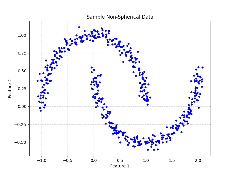
Figure 2: Sample non-spherical data

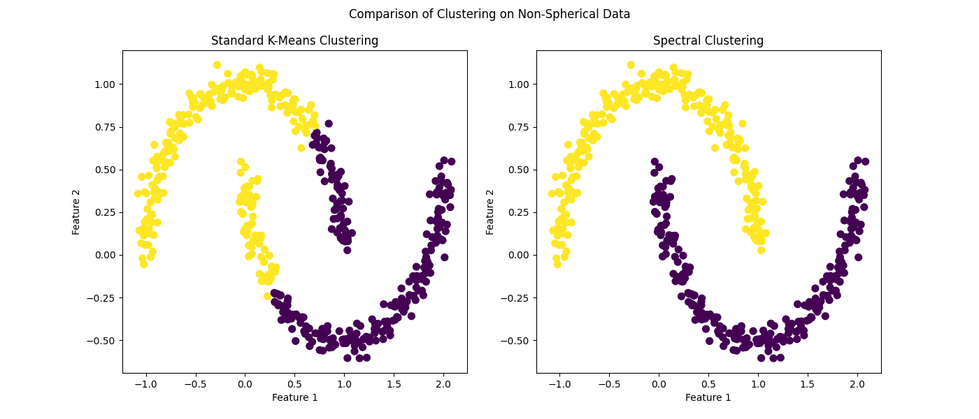
Figure 3: Comparison of clustering on non-spherical data

It hardly needs to be pointed out that spectral clustering — as a stand-in for kernel k-means — outperforms its standard counterpart in this scenario.

Wrapping Up

While the k-means algorithm is often introduced as a basic clustering technique, its utility extends beyond introductory examples. By incorporating a few clever approaches, we can overcome its most significant limitations and adapt it for the messy, complex nature of real-world data. These enhancements demonstrate that even foundational algorithms can remain highly relevant and powerful with the right modifications:

Using k-means++ for initialization provides a more robust starting point, leading to better and more consistent results.
The silhouette score offers a quantitative method for determining the optimal number of clusters, removing the guesswork from one of the algorithm’s key parameters.
Leveraging kernel methods through techniques like spectral clustering allows k-means to break free from its assumption of spherical clusters and identify intricate patterns in the data.

Don’t be so quick to dismiss k-means; by applying these practical techniques, you can unlock its full potential and gain deeper, more accurate insights from your data.

Source link